Bridge Deck Analysis By Finite Difference Method

A detailed analysis done by Gautam Chattopadhyay

Names and Symbols used:
Ardeck – area of the deck.
wdeck – width of deck.
span – span length of bridge.
izlong – Moment of inertia of each longitudinal girder about z axis (transverse axis)
iztrans – Moment of inertia of entire deck in transverse direction about longitudinal axis.
flexkl – Flexural rigidity in longitudinal direction.
flexkt – Flexural rigidity in transverse direction.
ngird – number of longitudinal girders.
tslong – Tosional rigidity in longitudinal direction.
tstrans – Torsional rigidity in transverse direction.
econc – modulus of elasticity of concrete.
gconc – shear modulus for concrete.
N (ndiv) – Number of divisions in either direction.

Bridge decks are normally comprised of a grillage system of longitudinal and transverse girders. Longitudinal girders are supported at two ends while the extreme edges in transverse direction remain free. Bridge decks need special methods of analysis when subjected to unsymmetrical loadings. Unsymmetrical loading occurs for the following reasons:

1. When one edge is provided with footpath and other end with crash barrier. Under such condition weight of crash barrier, weight of footpath and live load on footpath will exert asymmetric loads. In addition load due to wearing course will also become asymmetric.

2. Any vehicular live load is asymmetric.
The most common method of analysis for computing stress resultants is obtaining absolute bending moment and shearing force by using Influence Line Diagram (ILD) and then multiplying the values of stress resultants by respective distribution coefficients of longitudinal and transverse members. This method has long been practised by bridge design engineers. There are several methods of finding distribution coefficients which are being described below in brief:

1. Courban’s Method: Probably the oldest method of obtaining distribution coefficients. Courban treated the bridge deck as a rigid structure mounted over a number of rigid supports. Distribution formula is analogous to load distribution for a row of piles or bolts subjected to eccentric vertical load on the pile cap. This method gives fairly accurate results for decks having an aspect ratio between 2 and 4. Popularity of this method lies in its simplicity and the fact that most of the bridge decks we design come within the aspect ratio mentioned above.

2. Morrice – Little – Rowe method: computes distribution coefficients through close formed solution of governing differential equation of an equivalent anisotropic plate subjected to uniformly distributed load. This method seeks solution in trigonometric series as per M Levy’s method. M Levy suggested solution of the governing partial differential equation for plates having two opposite edges simply supported and the other two opposite edges of different definition, free for a bridge deck. The method is a generalized one and is applicable for any aspect ratio.

3. B N Baikov’s method: employs harmonic analysis to solve the problem. Harmonic analysis starts with an assumption that deflection of a beam “y” is a sine function of multiple of elementary span “x”.Thus

y=sin mpx/L where L is the span. p = pie = 3.14
Then rotation dy/dx works out to be mp/L cos mpx/L and d²y/dx² works out to be

–( mp/L)² sin mpx/L, or  d²y/dx² = –( mp/L)² y. d⁴y/dx⁴ thus becomes ( mp/L)⁴ y. This shows every even power of differential of deflection is a multiple of the deflection function itself. Recurrence of deflection function shows harmonic relation between bending moment and deflection. Similarly rotation and shear force are also proportional to each other and has a phase lag of 90⁰ with deflection and bending moment. The method of harmonic analysis was also suggested by Hendry and Jaegar. Baikov’s analysis has a clear distinction from others in the sense that provision of intermediate cross girders is not mandatory for analysis. He rather considered that deck slab offers sufficient lateral restrain to the longitudinal girders and considers that the deck slab is a plate on elastic foundation in shape of longitudinal girders. The method finally computes distribution coefficients by solving a set of simultaneous equations where number of equations is equal to the number of longitudinal girders. This method is also a generalized one and applicable to deck slab of any aspect ratio.

4. Finite Element Analysis: All the above methods have their own limitation and applicability. 3D soft-wares solve the problem of analyzing deck structure by finite element method where both longitudinal and cross girders are considered as beam elements assembled to form a space structure. A beam element in space has six degrees of freedom at each end. Stiffness matrix of a plane beam element is obtained by using displacement function which is a third degree polynomial in x,

y = Ax³ + Bx² + Cx + D
where x is an element of span of the beam. While assembling stiffness matrices of two consecutive beams, stiffness values at the connecting node are added up and boundary values depending on support characteristics are employed to formulate the global stiffness matrix. Load vector is prepared by applying external forces such as point loads, moments, torsion as per the conditions of analysis. Force vector consists of fixed end forces due to loads applied on a beam element. Finite element method being basically a stiffness method seeks displacement of the deck structure under application of external forces. Bending moments, torsion and shearing forces are then computed using slope – displacement relations. Soft-wares like STAAD, SAP, PASFEM etc, follow Finite Element Method of analysis.

A brief description of Finite Element Method
A brief introduction to FEM is being presented here with special reference to beam element only since mainly beam element is used in bridge design.

Displacement Function of a 2D beam element is given by:
y = Ax³ + Bx² + Cx + D.
Hence, dy/dx = 3Ax² + 2Bx + C.
Boundary conditions are:
y=v_i at x = 0 and v_j at x = L
dy/dx = q_i at x = 0 and q_j at x = L

Therefore D = v_i and C = q_i.
Solving for remaining coefficients A and B we obtain,
y =  [2(x/L)³ – 3(x/L)² + 1] v_i +[3(x/L)² – 2(x/L)³] v_j + [1 – 2L(x/L)² + L(x/L)³] q_i + L[(x/L)³ – (x/L)²] q_j.

If we apply v_i = 1 keeping all other displacements at zero, we get
y = [2(x/L)³ – 3(x/L)² + 1].

This function is called Shape Function for displacement v_i and describes the shape of the displacement v_i along length of the beam element ij. Similar shape functions can be obtained for all other displacements by putting 1 for that particular displacement and zero for others.

In a similar manner displacement function of a plate is expressed as:
w(x,y) = A₁ + A₂x + A₃y + A₄x² + A₅xy + A₆y² + A₇x³ + A₈x²y + A₉xy² +A₁₀y³ + A₁₁x³y + A₁₂xy³.

Suggesting there are 12 unknown degrees of freedom. The degrees of freedom are one vertical displacement and two rotations at each of the four nodes of a plate.

Shape functions for each of these displacements can be derived in the same manner as elaborated for beam element

Elements of Stiffness matrix in local coordinate system is then derived by integrating products of shape functions from 0 to L of the particular member.

Local member stiffness matrix is then multiplied by geometry matrix which describes orientation of the element and consists of direction cosines of the element. A unique property of this matrix is its inverse is equal to its transpose.

The product thus obtained is then multiplied by transpose of the geometry matrix to obtain stiffness matrix of a beam element in global coordinates.

Global Stiffness Matrices of all the elements are then assembled to represent the entire structure.

The fundamental static equilibrium equation of a structure is [K] {x} = {P} where [K] is the stiffness matrix and {x} and {P} are displacement vector and Force Vector respectively. {x} may consist of all unknown displacements like axial displacement, vertical displacement, rotations about axes. {P} consists of fixed end forces and computed by obtaining Fixed End Moments, Shears etc, due to the loads applied on various beam elements.   

Analysis By Other Methods:
Present paper suggests a different approach towards computing distribution coefficients and stress resultants.

Like Morrice Little or B N Baikov this method also seeks solution of basic partial differential equation for an orthotropic grillage system but instead of seeking close – formed solution the method solves the fundamental equation using method of finite differences.

The governing partial differential equation for an orthotropic grillage system is given by:

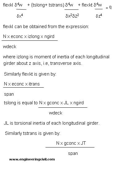
Here JT is total torsional inertia in transverse direction, i.e, sum of torsional inertias of the cross girders and that of remaining portion of deck slab.

The multiplier N appearing in the expressions above is because span and width of the deck have been divided into N equal parts for ease of forming difference equations.

q (x,y) is the load function to which the grillage system is subjected.

Method of Finite Differences
Method of finite difference is a mathematical tool used to solve differential equations, both total and partial, by forming difference equations at nodal points. A set of simultaneous equations thus obtained is solved by matrix algebra. The method is simple and though approximate, gives results accurate enough for practical design purposes.

Every differential dy/dx or its higher orders can be expressed in terms of difference equations which transforms solution of differential equation into an algebraic problem. A few illustrations, which are also available in text books of higher mathematics being presented here:
dy/dx = (y_i – y_i+1)/h

Where y represents ordinates of a function at i^th, (i+1)^th points and h is interval between x_i and x_i+1. This is called forward difference. Similarly for backward difference i is to be replaced by i-1 and i+1 by i. Thus summing up the two expressions thus obtained, central difference for first order differential is given by:

dy/dx     ₌ (y_i-1 – y_i+1)/2h
which is called central difference.

Differentiating this expression further with respect to x means writing difference equations for each of y_i-1 and y_i+1. Thus

d²y/dx² h=  [ (yi-1 – yi)/h – (yi – yi+1)/h]/h
or,
d²y/dx^{2 =} [y_i-1 – 2y_i+ y_i+1]/h2

Expressions can be extended further to obtain third order, fourth order and even higher orders of differentials. We shall use Taylor’s Series to obtain difference expressions of higher order as shown below:

By Taylor’s Series,
f(x+h)= f(x) + hf’(x) + h²/2 f”(x) + h³/6 f”’(x) + h⁴/24 f^iv(x). ………(i)

The terms of higher order differentials are being neglected.
By substituting h by – h in the above expression we obtain
f(x-h)= f(x) – hf’(x) + h²/2 f”(x) – h³/6 f”’(x) + h⁴/24 f^iv(x)……..(ii)

Therefore,
f(x+h) – f(x-h) = 2h f’(x) + h³/3 f”’(x)……….(iii)
Substituting h by 2h in above expression we find
f(x+2h) – f(x-2h) = 4h f’(x) + 8h³/3 f”’(x)……….(iv)
but, from expression (iii), 4hf’(x) = 2f(x+h) – 2f(x – h) – 2h³/3 f”’(x).
Therefore f(x+2h) – f(x-2h) = 2f(x+h) – 2f(x – h) – 2h³/3 f”’(x) + 8h³/3 f”’(x).
or, f(x+2h) – 2f(x+h) + 0. f(x) + 2f(x-h) – f(x – 2h) = 2h³ f”’(x)……..(v)

Thus, in our terminology,
d³y/dx3    is given by  [-y_i-2 + 2y_i-1 – 2y_i+1 + y_i+2]/2 h³

again, by adding up expressions (i) and (ii) we obtain,
f(x+h) + f(x – h) = 2f(x) +h²f”(x) + h⁴/12 fiv(x)……..(vi)
Substituting h by 2h in above expression we find
f(x + 2h) + f(x – 2h) = 2f(x) +4h²f”(x) + 16h⁴/12 f^iv(x)……(vii)
Hence, 4h²f”(x) = f(x + 2h) + f(x – 2h) – 2f(x) – 16h⁴/12 f^iv(x)……..(viii)
Putting expression (viii) in expression (vi) we obtain
4f(x+h) + 4f(x – h) = 8f(x) + f(x + 2h) + f(x – 2h) – 2f(x) – 16h⁴/12 f^iv(x) + 4h⁴/12 f^iv(x).
Or,
h⁴f^iv(x) = f(x + 2h) – 4f(x + h) + 6f(x) – 4f(x – h) + f(x – 2h)……(ix)
Therefore,
f^iv(x)= {f(x + 2h) – 4f(x + h) + 6f(x) – 4f(x – h) + f(x – 2h)}/h⁴…….(x)
Or, in our terminology,
d⁴y /dx^{4 =[} y_i-2 – 4y_i-1 + 6y_i – 4y_i+1 + y_i+2]/h⁴

To obtain the torsion terms like d²w/dxdz we shall deduce the difference expressions from fundamentals. The most familiar method of solving partial differential equations in two variables is expressing the equation as a product of two independent functions:

Then, w(x,z) = f(x)g(z)
Hence d⁴w/dx²dz² = f”(x)g”(z)
Since f(x) and g(z) are functions of x and z only we can write
d⁴w/dx²dz² = (w_x-1 – 2w + w_x+1)/h_x² x (w_z-1 – 2w + w_z+1)/h_z²

Hence it comes out that,
d⁴y /dx²dy2=[y_(i+1,j-1) – 2y_(i+1,j) + y_(i+1,j+1) – 2y_(i,j-1) + 4y_(i,j) – 2y_(i,j+1) + y_(i-1,j-1) – 2y_(i-1,j) + y_(i-1,j+1)]/
h_x²h_z²

Expression for d³w/dx²dz can be obtained by noting that
d³w/dx²dz = f”(x)g(z).

Thus we can express the differentials in terms of finite difference expansions, i.e, algebraic expressions in the following way:

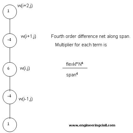
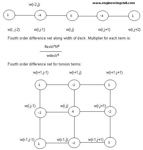
Each term is to be multiplied by:
[(tslong + tstrans)*N4]/(ardeck)2

Thus when arranging the difference equation for a particular node (I,j) it becomes as follows:

displacement	coefficient
w(i,j)	(6*(flexkl/span4 + flexkt/wdeck4) + 4*( tslong + tstrans)/ardeck2)*N4
w(i,j-1)	-(4* flexkt/wdeck4 + 2*(tslong + tstrans)/ (ardeck)2)*N4
w(i+1,j)	-(4* flexkl/span4 + 2*(tslong + tstrans)/ (ardeck)2)*N4
w(i-1,j)	-(4* flexkl/span4 + (tslong + tstrans)/ (ardeck)2)*N4
w(i,j-1)	-(4* flexkt/wdeck4 + 2*(tslong + tstrans)/ (ardeck)2)*N4
w(i,j+1)	-(4* flexkt/wdeck4 + 2*(tslong + tstrans)/ (ardeck)2)*N4
w(i+2,j)	flexkl/span4*N4
w(i+1,j-1)	(tslong + tstrans)*N4/(ardeck)2
w(i-1,j-1)	(tslong + tstrans)*N4/(ardeck)2
w(i+1,j+1)	(tslong + tstrans)*N4/(ardeck)2
w(i-1,j+1)	(tslong + tstrans)*N4/(ardeck)2
w(i-2,j)	flexkl/span4*N4
w(i,j+2)	flexkt/wdeck4*N4
w(i,j-2)	flexkt/wdeck4*N4

Thus every node is sharing some flexural as well as twisting effect from neighboring nodes, a phenomenon very similar to “Carry Over” in frame analysis. Thus partial differential equation at a general intermediate node (i,j) takes the following shape:

[(6*(flexkl/span⁴ + flexkt/wdeck⁴) + 4*( tslong + tstrans)/ardeck²)*N⁴]w_ij + -{(4* flexkt/wdeck⁴ + 2*(tslong + tstrans)/ (ardeck)²)}*N⁴ w_(i+1,j) + -{(4* flexkl/span⁴ + 2*(tslong + tstrans)/ (ardeck)²)*N⁴} w_(i-1,j) + flexkl/span⁴*N⁴ + flexkt/wdeck⁴*N⁴ = q

Thus equations will be prepared for every node which will form the global stiffness matrix for vertical displacement of the grillage system.

Boundary conditions:

1. At simply supported nodes w is zero. So also is d²w/dx² + nd²w/dz² where n is Poisson’s Ratio and taken to be -0.15 for concrete.
2. At fixed nodes w is zero and dw/dz or dw/dx is zero.
3. At free nodes both bending moment and shear force will be zero. Hence,

d²w/dx² + nd²w/dz² = 0 and also, d³w/dx³ + (2 – n) d³w/dxdz² = 0 along axis of x and by replacing x by z we get expression of shear along axis of z.

Since a bridge deck consists of free edges at the extremities along transverse direction boundary conditions for free nodes are to be applied.

Since at free edge bending moment and shearing forces do not exist, displacement of every node on free edge must follow the expressions:

d²w/dx² + nd²w/dz² = 0 and

d³w/dx³ + (2 – n) d³w/dxdz² = 0.

From expressions shown above it is obvious that difference equation at a node in vicinity of boundary will extend beyond to the boundary line. As an example, fourth order difference expression will extend beyond boundary by two exterior nodes. Thus we shall have to consider some fictitious nodes outside the boundary of the plate which will be eliminated by establishing their relations with nodes within the plate boundary by using boundary conditions.

Since nodes on free edge will undergo deflection which we shall have to determine, difference equations at these nodes will extend beyond the boundary of the plate by two nodes. Thus we shall have to consider two fictitious boundaries.

We shall now illustrate the method through a small example where distribution coefficients at girders of a bridge deck having a span of 33 m and a deck width of 12 m will be investigated into. The deck has four longitudinal girders and five cross girders.

THE GEOMETRIC MODEL

The dashed boundary lines at two edges of the deck structure denote free edges. There are two dashed lines beyond either of the transverse edges to accommodate the fictitious nodes required for boundary conditions. Such fictitious boundary is also shown beyond each of the longitudinal extremities to accommodate fictitious nodes required to satisfy boundary conditions. It may be noted that no fictitious node is assumed along simply supported edges of the deck. This is because of following reason:

Let us assume a node 150 on left hand side of 1. Since 1 is part of simply supported edge, both w₁ and M_x1 should be zero. Similarly w₂ should also be 0. Hence,

w₁₅₀ – 2 w₁ + w₂ = 0. Proving that w₁₅₀ is also 0.

In the mesh it is obvious that being nodes on simply supported edge,

w₁ to w₁₁ and w₁₂₂ to w₁₃₂ will not undergo any displacement. Hence writing difference equations for these nodes is not needed.

Developing Stiffness Matrix

Stiffness matrix is developed by preparing equations at each node individually. Let us write difference equation at node no. 15:

{6*(flexkl/span⁴ + flexkt/wdeck⁴) + 2*( tslong + tstrans)/ardeck²}*N⁴w₁₅ + -{4* flexkl/span⁴ + 2*(tslong + tstrans)/ (ardeck)²}*N⁴ w₄ + -{4* flexkl/span⁴ + 2*(tslong + tstrans)/ (ardeck)²)*N⁴} w₂₈ + -{4* flexkt/wdeck⁴ + 2*(tslong + tstrans)/ (ardeck)²}*N⁴ w₁₄ +-{4* flexkt/wdeck⁴ + 2*(tslong + tstrans)/ (ardeck)²}*N⁴ w₁₆ + (tslong + tstrans)*N⁴/(ardeck)² w₃ + (tslong + tstrans)*N⁴/(ardeck)²w₅ +(tslong+tstrans)*N⁴/(ardeck)² w₂₇ + (tslong + tstrans)*N⁴/(ardeck)² w₂₉ + flexkl*N⁴/ span⁴ w₁₇₉ + flexkl*N⁴/ span⁴ w₄₁ + flexkt*N⁴/ wdeck⁴ w₁₃ + flexkt*N⁴/ wdeck⁴ w₁₇ = q₁₅

The terms containing w₃,w₄ and w₅ readily vanish as these deflections are zero. Now applying the second boundary condition that d²w/dz² at node 4 is zero, we get in terms of deflections:

W₅₀₆ – 2w₄ + w₁₅ = 0.

Since w₄ itself is zero, w₁₅ = – w₅₀₆

Thus coefficient of w₁₅ in the above equation becomes:

(6*(flexkl/span⁴ + flexkt/wdeck⁴) + 4*( tslong + tstrans)/ardeck² – flexkl / span⁴)*N⁴.

The final shape of the equation now is:

(5*flexkl/span⁴ + 6*flexkt/wdeck⁴ + 4*(tslong + tstrans)/ardeck²)*N⁴ w₁₅ – (4* flexkl/span⁴ + 2*(tslong + tstrans)/ (ardeck)²)*N⁴ w₂₈ – (4* flexkt/wdeck⁴ + 2*(tslong + tstrans)/ (ardeck)²)*N⁴ w₁₄ – (4* flexkt/wdeck⁴ + 2*(tslong + tstrans)/ (ardeck)²)*N⁴ w₁₆ +(tslong + tstrans)*N⁴/(ardeck)² w₂₇ + (tslong+tstrans)*N⁴/(ardeck)² w₂₉ + flexkl*N⁴/ span⁴ w₄₁ + flexkt*N⁴/ wdeck⁴ w₁₃ + flexkt*N⁴/ wdeck⁴ w₁₇ = q₁₅

Thus equation for w₁₅ is now formed. Band width of this equation is 29, which can be reduced by renumbering the nodes.

We can also see that w₁₃ to w₁₉ are equal to – w₁₇₇ to – w₁₈₃ respectively. Similarly w₁₀₃ to w₁₁₁ are equal to – w₅₀₃ to – w₅₁₀ respectively.

Let us now concentrate on node no. 13. The difference equation will be:

(6*(flexkl/span⁴ + flexkt/wdeck⁴) + 4*( tslong + tstrans)/ardeck²)*N⁴ w₁₃ + -(4* flexkl/span⁴ + 2*(tslong + tstrans)/ (ardeck)²)*N⁴ w₂ + -(4* flexkl/span⁴ + 2*(tslong + tstrans)/ (ardeck)²)*N⁴ w₂₆ + -(4* flexkt/wdeck⁴ + 2*(tslong + tstrans)/ (ardeck)²)*N⁴ w₁₂ +-(4* flexkt/wdeck⁴ + 2*(tslong + tstrans)/ (ardeck)²)*N⁴ w₁₄ + (tslong + tstrans)*N⁴/(ardeck)² w₁ + (tslong + tstrans)*N⁴/(ardeck)² w₃ +(tslong + tstrans)*N⁴/(ardeck)² w₂₅ + (tslong + tstrans)*N⁴/(ardeck)² w₂₇ + flexkl*N⁴/ span⁴ w₁₇₇ + flexkl*N⁴/ span⁴ w₃₉ + flexkt*N⁴/ wdeck⁴ w₁₁ + flexkt*N⁴/ wdeck⁴ w₁₅ = q₁₃.

From this expression we delete the zero deflection terms w₁, w₂ and w₃. Again w₁₇₇ is – w₁₃. Therefore the expression reduces to:

(6*(flexkl/span⁴ + flexkt/wdeck⁴) + 4*( tslong + tstrans)/ardeck² – flexkl / span⁴)*N⁴ w₁₃ – (4* flexkl/span⁴ + 2*(tslong + tstrans)/ (ardeck)²)*N⁴ w₂₆ + -(4* flexkt/wdeck⁴ + 2*(tslong + tstrans)/ (ardeck)²)*N⁴ w₁₂ +-(4* flexkt/wdeck⁴ + 2*(tslong + tstrans)/ (ardeck)²)*N⁴ w₁₄ + (tslong + tstrans)*N⁴/(ardeck)² w₂₅ + (tslong + tstrans)*N⁴/(ardeck)² w₂₇ + flexkl*N⁴/ span⁴ w₃₉ + flexkt*N⁴/ wdeck⁴ w₁₁ + flexkt*N⁴/ wdeck⁴ w₁₅ = q₁₃.

The expression still contains a fictitious deflection w₁₁. To eliminate this fictitious term we now apply the condition that d²w/dx² is zero at node 12.

Therefore, w₁₁ – 2 w₁₂ + w₁₃ = 0.

Now we substitute 2 w₁₂ – w₁₃ for w₁₁. Hence the difference equation at node 13 finally takes the following shape:

(6*(flexkl/span⁴ + flexkt/wdeck⁴) + 4*(tslong + tstrans)/ardeck² – flexkl / span⁴– flexkt/ wdeck⁴)*N⁴ w₁₃ – (4* flexkl/span⁴ + 2*(tslong + tstrans)/ (ardeck)²)*N⁴ w₂₆ + -(4* flexkt/wdeck⁴ + 2*(tslong + tstrans)/ (ardeck)² + 2*flexkt/ wdeck⁴)*N⁴ w₁₂ +-(4* flexkt/wdeck⁴ + 2*(tslong + tstrans)/ (ardeck)²)*N⁴ w₁₄ + (tslong + tstrans)*N⁴/(ardeck)² w₂₅ + (tslong + tstrans)*N⁴/(ardeck)² w₂₇ + flexkl*N⁴/ span⁴ w₃₉ + flexkt*N⁴/ wdeck⁴ w₁₅ = q.

– which does not contain any fictitious node. Similar expression will be obtained for node number 19 also. Because of the presence of boundary node no. 12, band width of the expression rises to 28. Difference equations can be easily formulated for nodes 41, 42, 43 etc, where the difference trees will not extend beyond boundary of the plate.

The boundary conditions may also be treated as additional equations but it is better to apply them manually before forming the matrix. Additional equations will unnecessarily increase size of the matrix affecting computation time and accuracy. The more is the number of equations, more is the triangulation error.

We shall now discuss difference equation at node no. 12. Node no. 12 is located on free edge and hence is free to deflect. Because its difference network extends up to two fictitious boundaries the equation will include four fictitious nodes which will have to be eliminated by using boundary conditions at a free edge.

Let us first write difference equation at 12 and then eliminate fictitious and other unnecessary terms in following way:

(6*(flexkl/span⁴ + flexkt/wdeck⁴) + 4*( tslong + tstrans)/ardeck²)*N⁴ w₁₂ + -(4* flexkl/span⁴ + 2*(tslong + tstrans)/ (ardeck)²)*N⁴ w₁ + -(4* flexkl/span⁴ + 2*(tslong + tstrans)/ (ardeck)²)*N⁴ w₂₅ + -(4* flexkt/wdeck⁴ + 2*(tslong + tstrans)/ (ardeck)²)*N⁴ w₁₁ +-(4* flexkt/wdeck⁴ + 2*(tslong + tstrans)/ (ardeck)²)*N⁴ w₁₃ + (tslong + tstrans)*N⁴/(ardeck)² w₁₅₀ + (tslong + tstrans)*N⁴/(ardeck)² w₂ + (tslong + tstrans)*N⁴/(ardeck)² w₂₄ + (tslong + tstrans)*N⁴/(ardeck)² w₂₆ + flexkl*N⁴/ span⁴ w₁₅₁ + flexkl*N⁴/ span⁴ w₃₈ + flexkt*N⁴/ wdeck⁴ w₁₀ + flexkt*N⁴/ wdeck⁴ w₁₄ = q.

In this expression two fictitious nodes 150 and 151 have been introduced where w is zero as shown earlier. Thus we find w₁ = w₂ = w₁₅₀ = w₁₅₁ = 0.

Hence equation reduces to:
(6*(flexkl/span⁴ + flexkt/wdeck⁴) + 4*(tslong + tstrans)/ardeck²)*N⁴ w₁₂ – (4* flexkl/span⁴ + 2*(tslong + tstrans)/ (ardeck)²)*N⁴ w₂₅ – (4* flexkt/wdeck⁴ + 2*(tslong + tstrans)/ (ardeck)²)*N⁴ w₁₁ +-(4* flexkt/wdeck⁴ + 2*(tslong + tstrans)/ (ardeck)²)*N⁴ w₁₃ + (tslong + tstrans)*N⁴/(ardeck)² w₂₄ + (tslong + tstrans)*N⁴/(ardeck)² w₂₆ + flexkl*N⁴/ span⁴ w₃₈ + flexkt*N⁴/ wdeck⁴ w₁₀ + flexkt*N⁴/ wdeck⁴ w₁₄ = q.

We now have to eliminate deflections at fictitious nodes namely w₁₀, w₁₁ and w₂₄. The boundary conditions are:
w₁₁ – 2w₁₂ + w₁₃ = 0.
– w₁₀ + 2w₁₁ – 2w₁₃ + w₁₄ = 0. (Please refer to page 6 for d³y/dx³).

Putting value of w11 from first expression in second expression we obtain:
w₁₀ – 2*(2w₁₂ – w₁₃) + 2w₁₃ – w₁₄ = 0.or,
w₁₀ – 4w₁₂ +2w₁₃ + 2w₁₃ – w₁₄ = 0.
Or, w₁₀ – 4w₁₂ + 4w₁₃ – w₁₄ = 0.
Or, w₁₀ = 4w₁₂ – 4w₁₃ + w₁₄.

Thus terms w₁₀ and w₁₁ can now be readily eliminated by substituting these expressions. The next fictitious deflection at 24 can be eliminated by writing:

w₂₄ = 2w₂₅ – w₂₆. This eliminates all fictitious deflections from the difference equation at node 12. Band width of this equation however reduced a bit – 27.
Difference equations at all the nodes can thus be generated.

The unknown part of these equations comprises of a vector of unknown vertical deflections. Please note by adopting finite difference method we are generating a stiffness matrix of the given grillage corresponding to vertical deflections at various nodes. Coefficients of deflections form a square matrix which is stiffness matrix of the grillage in global coordinate system. Thus we have generated a stiffness matrix of the structural system corresponding to vertical deflections only.

Generating Load Vector:
While preparing load vector it must be born in mind that Kirchoff’s equation of equilibrium of a plate – the entire formulation is based is for plate subjected to uniformly distributed load only. If there be line load or concentrated load acting on a small area, the trigonometric series is to be considered in a different manner: series for loaded portion of the plate and that for unloaded portion. Therefore the load vector should contain only UDLs or pressures at various nodes and not concentrated loads. This prohibition is also evident from unit of the terms in stiffness matrix.

In order to prepare the load vector, the wheel loads are to be divided by their respective effective areas i.e, product of effective width and length. Depending on position of the load, the pressure thus obtained will be distributed between four adjacent nodes. Thus while some nodes will be subjected to pressure due to wheel load, other nodes will not be subjected to any load at all.

Positions of wheel loads are determined for maximum bending moment at mid span using influence line diagram of bending moment at mid span.

The following calculations show maximum absolute bending moment at mid span due to class A wheel load and class 70 R wheel loads for a bridge deck of span 33 m and width of 12 m:

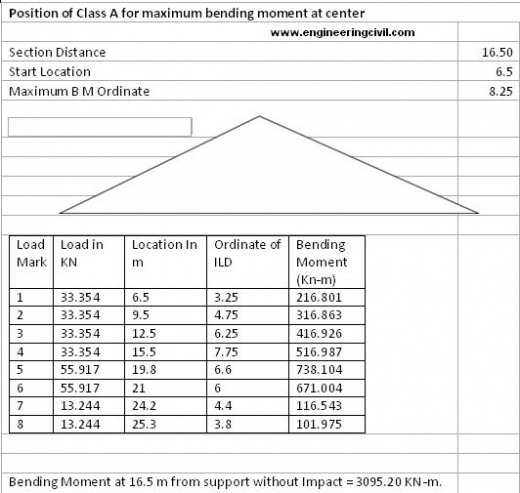
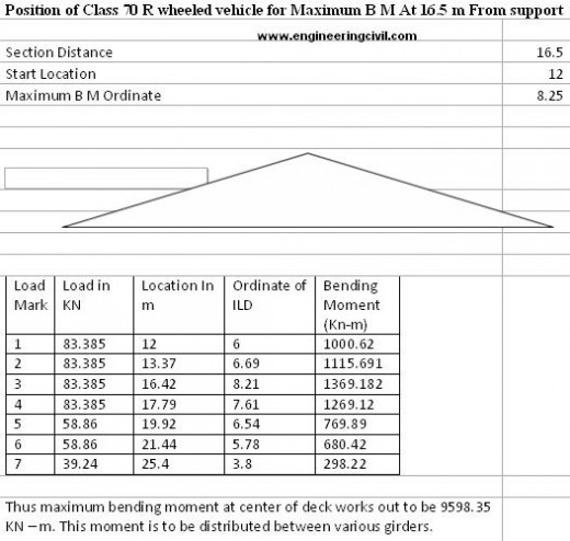
The class A wheel loads have been placed 0.9 m from edge of deck considering 0.5 m wide crash barrier. Thus second train of class A is at 2.7 m from left hand edge. The left hand train of class 70 R wheels will be at 4.58 m from left hand edge of deck and finally right hand train of class 70 R wheeled vehicle shall be at 6.51 m from left hand edge.

The nodal pressures form load vector and equation [K]{x}={p} is then solved by using MS Excel. Nodal displacements thus obtained are being shown in forms of graphs.

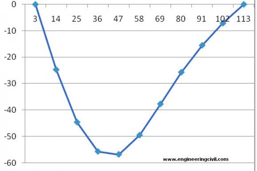
Displacements of nodes along central transverse axis of the deck slab are shown in figure 1.

Node 56 being on free edge has undergone maximum downward deflection. The upward deflections at 65 and 66 indicate effect of loads close to the left hand side. Distribution coefficients may also be computed by measuring the deflections at girder locations.

Girders are located between nodes 57 and 58 where displacements are 61.1 mm and 49.5 mm respectively. Displacement at location of girder has to be interpolated.

Thus displacements can be evaluated at locations of girders, both outer and inner. Stress Resultants like Bending Moment, Shear forces etc, can then be readily computed from nodal deflections.
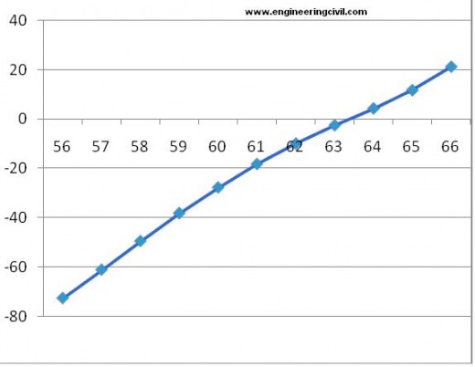
Figure 2 shows displacements along free edge:

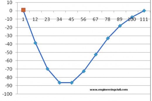
Figure 3 shows displacement along longitudinal axis at 1.2 m (width of deck/number of divisions) away from left free edge of the deck:

Maximum deflection occurs at node 57 and numerically -72 mm.

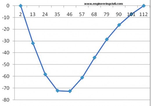
Figure 4 below shows deflections of nodes along a longitudinal axis at 2.4 m from left outer edge:

Referring to figure 1, displacements at girder locations have been determined by interpolating linearly between displacements of neighboring nodes as shown in table below.

Girder marks	Girder 1	Girder 2	Girder 3	Girder 4
Displacements at midspan (mm)	-61.1	-46.2	-32.1	-18.0

These displacements are then divided by central displacement of a beam having same EI and subjected to concentrated loads due to class A and class 70 R vehicles. The ratios are then normalized and the following distribution coefficients have been computed:

	Girder 1	Girder 2	Girder 3	Girder 4
By F D M	0.407	0.308	0.214	0.12
By Courban	0.446	0.315	0.185	0.054

Bending moments multiplied by respective distribution factors at mid span of various girders are determined and compared with other methods:

Girder Mark	B M by F D analysis in Kn-m	B M by STAAD in Kn-m	B M by Couban’s factor in Kn-m
Girder 1	– 3907.64	– 3776.77	– 4280.87
Girder 2	– 2954.71	– 2959.98	– 3023.38
Girder 3	– 2052.95	– 2082.22	– 1775.70
Girder 4	-1151.19	-1130.64	– 518.31

Table below shows the deflections of various girders at centre of span and compares them with deflections computed by STAAD:

Girder Mark	Deflections obtained F D analysis in mm	Deflections obtained by STAAD in mm
Girder 1	-61.1	-76.2
Girder 2	-46.2	-62.04
Girder 3	-32.1	-35.49
Girder 4	-18	-25.90

Conclusion:
1. Results obtained by finite difference analysis do not differ much from those obtained by FEM for left hand outer girder. Even then one should admit the facts that:

a) Finite difference method is an approximate solution since it ignores higher order terms.

b) Poisson’s effect has not been considered throughout the formation of stiffness matrix. In fact Poisson’s effect has been neglected in the basic differential equation of equilibrium. Therefore the output is definitely on higher side.

c) Deflections at locations of girders have been obtained by linear interpolation. Actual shape of deflection curve being parabolic, this adds further to approximation.

d) The outer girder is close to the free edge. FDM treats free edge as a set of nodes at which bending moment and shear force will be zero and computes all other nodal displacements on that basis. In FEM model, provision of edge beam is mandatory. Thus edge of the bridge deck carries some bending moment which is not available in FDM. Central girder does not undergo any effect of the free edge and stress resultants at inner girders are almost equal to that obtained from FEM.

e) Deflections obtained by FDM are quite fairly comparable to those obtained by FEM. This is because, both FDM and FEM allows deflection at the free edges irrespective of existence of edge beams.

f) FDM, though highly theoretical, can be easily applied in solution of practical problems of bridge design. Now – a – days since digital computers are easily available and problems can be solved by using MS office application like MS Excel or MATLAB. Once one problem is solved, the file can be used repetitively for many other projects.

g) The model of FDM is unique and need not be changed every time for a new project. Displacements of girders may be interpolated between displacements of neighbouring nodes.

Finally, Even with so many simplifications, and approximations results obtained by finite difference method is fairly accurate for the purposes of practical design. The method though originally developed by Issac Newton himself, could not gain popularity among engineers probably because application of the method needs solution of a large number of simultaneous equations. In the past days, when there was no computer or, handy software to solve a high order of matrix equation by Gaussian elimination method no one might have been interested in applying the method. The days have considerably changed and high speed computers, in form of desk top and even lap tops are easily available now a day. Moreover, since MS Excel now provides excellent mathematical functions for solving high ordered matrix equations, I hope this age old method will be able to regain its due place in engineering applications.

The most valuable facility lies in the fact that the solution by this method can be embedded easily in an excel file of designing a deck structure and can be used repeatedly. The entire solution, including stiffness matrix, load vector and the resultant displacement vector will be accommodated within one worksheet of Excel 2007. Hence if dimensions of the deck have to be changed, the engineer will not have to run any software afresh. Fresh results can be obtained by changing the span and deck width in the data sheet. Since all the parameters are linked with each other, with change in any of the design parameters like, span, width of deck, number of girders and section properties the distribution coefficients will change automatically.

ANNEXURE
Bibliography
1. Rowe R E, Design of Reinforced concrete Bridges.
2. Baikov B N, Design of Concrete structures.
3. Timoshenko S and Winowsky Creiger S, Theory of Plates and Shells,
4. Bairagi N S, A Text Book of Plate Analysis.

We are thankful to Sir Gautam Chattopadhyay for posting this extremely important research paper here on engineeringcivil.com. We hope this paper will be of great help to the engineers who are looking for related researches in finite difference method

If you have a query, you can ask a question here.